Fitting the Curve
What I’m looking for is some sort of determination of “good picks” vs. “bad picks”. Luckily, through the miracle of hindsight, I already know how players performed through the length of the season. All I need now is an expected value: given a pick in the draft, and the position group that you’re looking for, what’s a reasonable expectation for points? This means, I need a function. In the simplest terms, a function is a single value of y for every value of x. Ideally, it needs to be continuous and it needs to be logical. I know exactly where to go for this… I need some trend lines.
The most common types of trend lines are exponential, linear, logarithmic, polynomial, power, and moving average. These are performative metrics, so I expect that there’s generally going to be a bigger point-spread among the top 5 RBs than between the 21st- and 25th-best RBs. That means, like most stats, I would expect a faster rate of decay at the start and a slower rate of decay at the end of our best-fit line. This immediately disqualifies linear. I’d also expect a slow decay to zero points as x approaches the higher numbers, and I don’t want to overfit the curve to the first few data points, so I am eliminating polynomial and moving average. For mathy reasons, I already expect that exponential or logarithmic will provide the best fit. Without getting too deep in the details (the math is easily handled by the NumPy package), I’ll spoil the surprise: logarithmic was the cleanest fit. With some simple NumPy calculations, I can find the functions and the R-squared values for each position group.


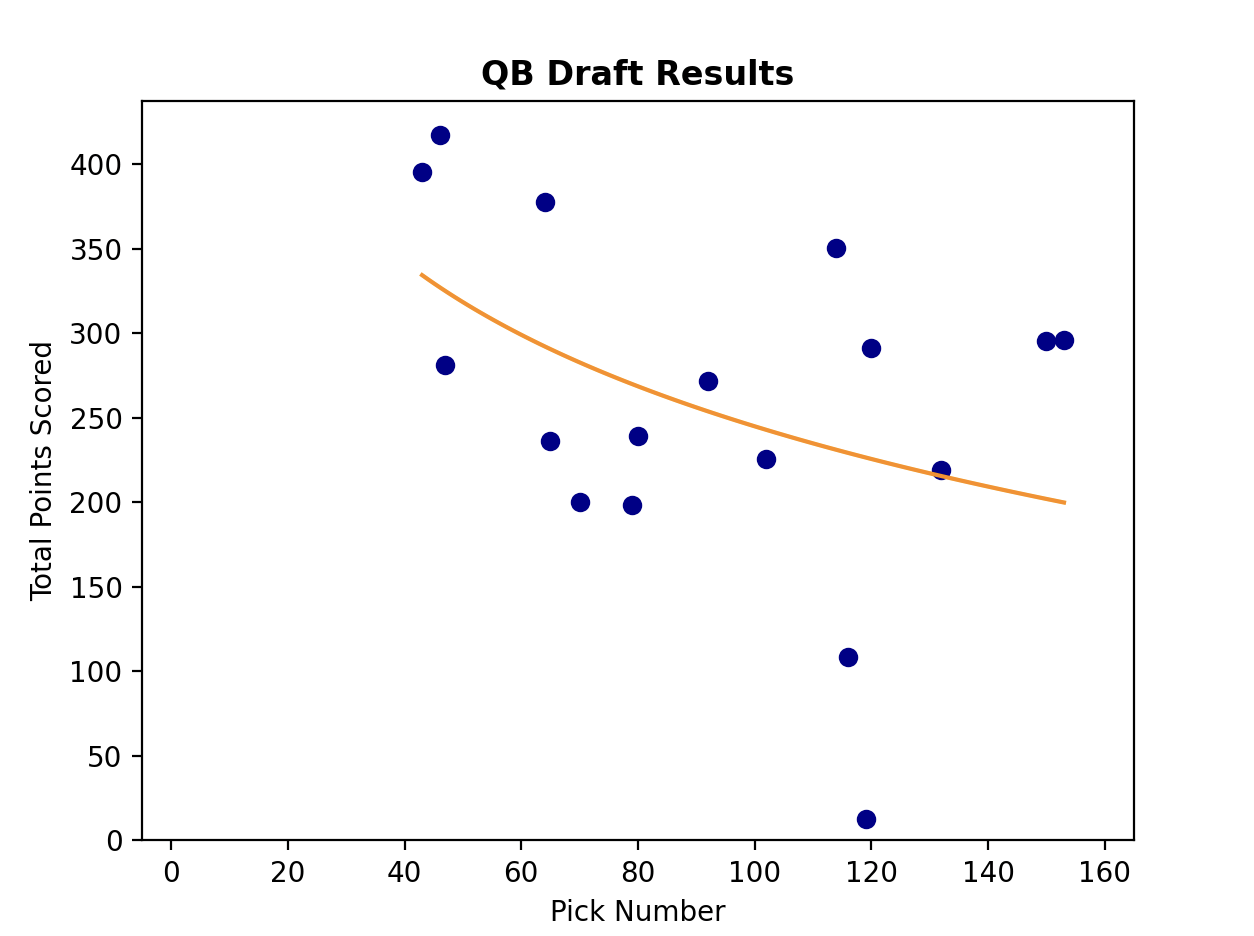
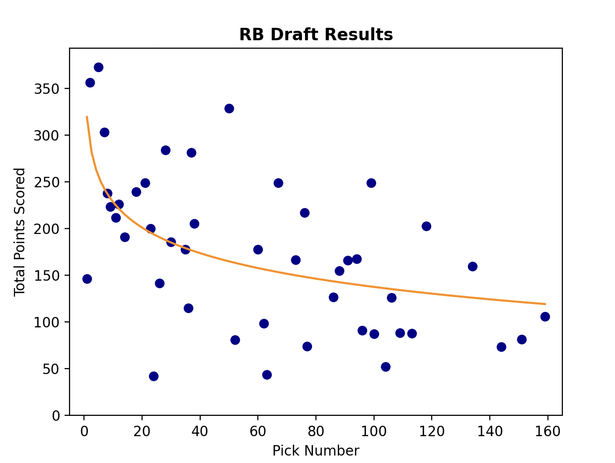
Before I overlay our new logarithmic trend lines with the scatter plots, it’s important to check the results against intuition. In the above formulas, I need to remember that y is an expectation for points scored over the season and x is the pick at which a player is drafted. Let’s assume that x=1, which means we are in the first pick of the draft. When x=1, ln(x)=0. That means, if we are drafting an RB with the first pick, we can reasonably expect 319 points (y = -39.46ln(1) + 319.24 = -39.46*0 + 319.24 = 319.24). That sounds about right; that’s a very high-performing RB. A WR drafted first could be expected to get 399 points. This also passes the general sniff test. But it looks like a QB drafted first should score…733? That wouldn’t only set a record for QBs all-time, that would be a 2-minute mile. 733 points would be a record that may never get broken.
It’s important to note here that our curve doesn’t necessarily represent how each player SHOULD be drafted. What it represents instead is, according to how our league drafted and how those players performed, 733 is a reasonable expectation for a QB that is drafted first overall. Because we waited until the fourth round to pick even the highest-rated QB, we are actually assigning a higher value to a QB that would be good enough to pick first overall. We are setting a much higher point-expectation for a QB than for a WR or RB who gets picked first. Is that smart? Not sure. But that’s one of the beautiful things about drafting. To be great at drafting, you don’t always pick the player who is going to score the most points first (if we did, we would always pick quarterbacks first). It’s the collective actions of the league that assign the value to players. I don’t want to spend a first-round pick on a QB in this league because I know that even the top QB will still be available when we get to the third round.
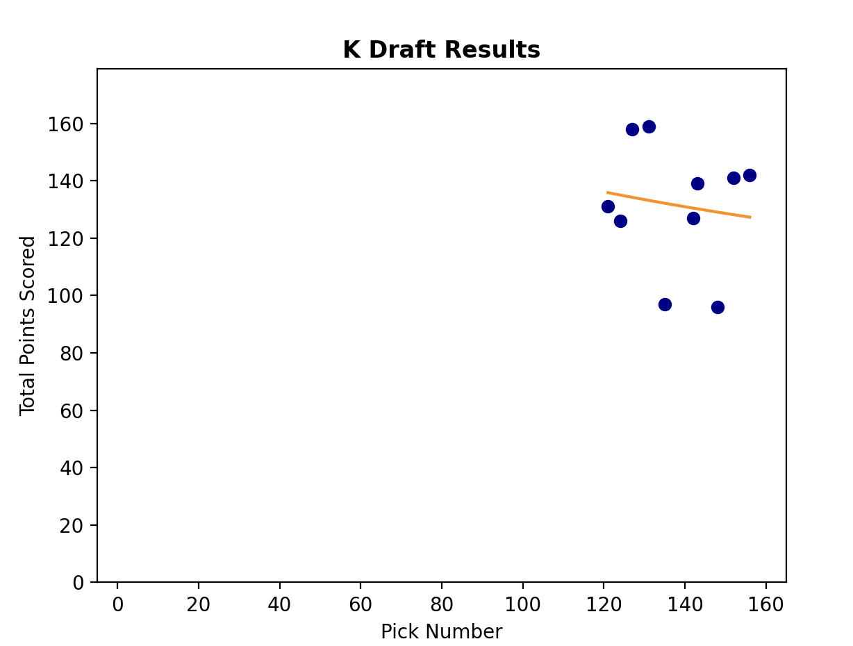
Another interesting piece of our NumPy functions is the R-squared value. This can generally be used as a metric for how well data fits the curve, and in our specific example, it’s a measurement of how confident we can be in our predictive skills for each position group. If we drafted perfectly for each position group, always drafting the top point-scoring RB before any others, we would fit the curves exceptionally well and our R-squared values would approach 1. But we aren’t perfect, and our R-squared values show it. Our R-squared value for WR was the highest, at .39, followed closely by RB and TE, both at about .34. This means that we were best able to predict WR scores, then RB and TE. Interestingly, our QB score was a very distant fourth, at .18. This is a finding that surprises me; intuitively, I would think that QBs would be the easiest position group to draft correctly. Defenses (D/ST) and Kickers had the lowest R-squared values by a MILE. This did not surprise me, and is a good reason why our league waits to pick them until the very latest rounds. When we did eventually start picking, we were essentially throwing darts. The R-squared values do indeed confirm a little bit of the rationale of our draft: we make our highest-confidence picks in the earliest rounds, because those are picks that we can’t afford to waste.
But enough of all that. With my best-fit curves ready to go, I’ll superimpose them on the previous scatter plots in hopes of finding the biggest wins and losses from last year’s draft.